

Visual EXPLAIN
Visual EXPLAIN turns raw execution plans into something you can actually work with. Select a query, click the EXPLAIN button, and Tabularis runs the appropriate EXPLAIN syntax for your database, parses the output, and presents it across six views — all without leaving the application.
Video unavailable
It works with PostgreSQL, MySQL, MariaDB, and SQLite, plus any plugin driver that declares EXPLAIN support. Each engine uses different EXPLAIN formats and capabilities, and Tabularis handles the differences automatically.
Try it in your browser — no install required. Paste any execution plan into Visual Explain Online and explore the same graph and table views at explain.tabularis.dev.
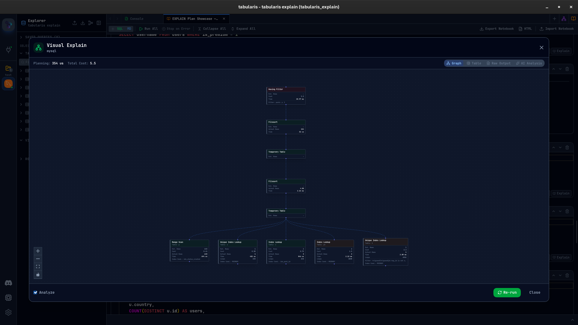
Opening Visual EXPLAIN
From the SQL Editor, select a query and click the EXPLAIN button in the toolbar to open the modal with the plan loaded.
Since v0.24.0, a Notebook SQL cell instead has a Show query plan button that opens an inline, resizable section. It first requests plain EXPLAIN, uses resolved notebook parameters and cell references, and can pop out into the full viewer without another request. Missing references prevent a request; changing the query, schema or connection marks the plan outdated until Re-run. See Notebook query plans.
The header shows the connection name, driver icon, database, and schema so you always know which server produced the plan.
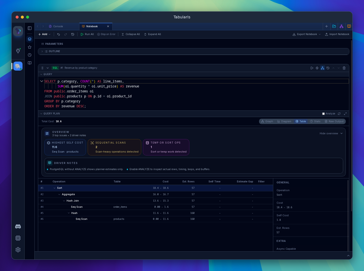
Which Queries Can Be Explained
Visual EXPLAIN accepts DML statements: SELECT, INSERT, UPDATE, DELETE, REPLACE, MERGE, WITH (CTEs), and TABLE.
DDL statements like CREATE, DROP, ALTER, and TRUNCATE are blocked — they are not valid inputs for EXPLAIN and would produce confusing errors from the database engine. If you try to explain a DDL statement, Tabularis shows an error message before anything is sent to the server.
SQL comments at the beginning of the query (both -- line comments and /* */ block comments) are stripped before validation, so annotated queries work as expected.
EXPLAIN vs EXPLAIN ANALYZE
A toggle in the modal footer switches between the two modes.
EXPLAIN shows the estimated plan — what the optimizer expects to happen. You get cost estimates, expected row counts, and the chosen access strategy, but nothing is executed.
EXPLAIN ANALYZE actually runs the query and reports what happened: actual row counts, actual execution time, loop counts, and (on PostgreSQL) buffer statistics. The difference can be significant — a plan might estimate 100 rows but actually scan 100,000.
In the standalone modal, the default depends on the query type:
| Query type | Default |
|---|---|
| Data-modifying statements (see below) | ANALYZE off, with a warning |
| Everything else (SELECT, read-only WITH, TABLE) | ANALYZE on |
Since v0.27.0 a statement counts as data-modifying when its first keyword, read after any leading comments and parentheses, is INSERT, UPDATE, DELETE, MERGE, REPLACE, UPSERT, TRUNCATE, CREATE, DROP, ALTER, GRANT, REVOKE, CALL, EXEC or EXECUTE, when it is a SELECT … INTO, or when a WITH statement contains INSERT, UPDATE, DELETE or MERGE outside strings and comments (a data-modifying CTE such as WITH deleted AS (DELETE … RETURNING …) SELECT …). For those, a warning icon appears next to the toggle, and since EXPLAIN ANALYZE executes the statement, you need to enable it explicitly. The choice is bound to the query, schema and connection rather than carried over to a new source.
The CTE check is a keyword scan, so it errs towards caution: a read-only CTE with a FOR UPDATE clause also opens with ANALYZE off, and you can tick it yourself. Side-effecting functions called from a SELECT are not detected; untick Analyze for those.
Notebook exception: the inline Query Plan section starts with plain EXPLAIN even for SELECT. Selecting Analyze does not run anything until you click Re-run. Its popout displays the already-fetched plan and has no separate execution controls.
Exclusive Metrics
Since v0.17.0, every node's figures are restated before any view renders. The database reports figures that are inclusive of children — and PostgreSQL's Actual Total Time is an average per loop — so ranking on the raw values always points at the plan root. Tabularis computes exclusive (self) metrics instead:
| Metric | Formula |
|---|---|
| Inclusive time | Actual Total Time × Actual Loops — a total, not a per-loop average |
| Exclusive time | inclusive time − Σ children's inclusive time |
| Exclusive cost | Total Cost − Σ children's Total Cost |
| Rows | Actual Rows × Actual Loops |
| Buffers | shared hits + reads, inclusive and exclusive |
| Time share | exclusive time ÷ plan total |
Graph nodes, the table view, and the overview bar rank and colour on these values — by exclusive time when the plan ran with ANALYZE, by exclusive cost otherwise. A node executed 50,000 times at 0.2 ms each is finally ranked above a node that ran once for 20 ms.
Per-Node Findings
Diagnostic checks run on every node and surface as labelled chips on the graph, icons in the table and diagram rows, and one-line explanations in the node details panel:
- Hotspot — the node accounts for ≥ 25% of total plan time and takes at least 1 ms
- More/fewer rows than planned — the optimizer's estimate is off by ≥ 4x (warning) or ≥ 10x (critical); skipped for nodes with fewer than 10 actual rows
- Sorted on disk — the sort spilled out of memory, or the node wrote temporary blocks
- Filter discards most rows — ≥ 90% of rows read are thrown away, and at least 1,000 rows are discarded
- Large sequential scan — a seq/full scan of ≥ 10,000 rows
- Many heap fetches (1,000 or more), fewer workers than planned, executed many times (≥ 1,000 loops), read from disk (≥ 50% of block accesses missed shared buffers, with at least 1,000 blocks read from disk), and never executed
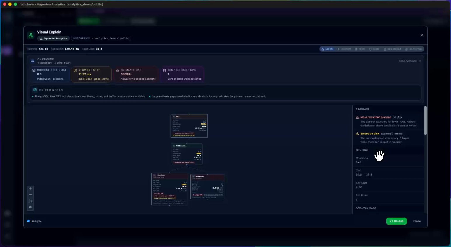
The Six Views
The summary bar at the top provides six tabs. You can switch views without re-running the query.
Graph View
The default view. Each operation in the plan becomes a node in an interactive directed graph. Seq Scan, Index Scan, Hash Join, Nested Loop, Sort, Aggregate — the full tree is rendered with edges showing the data flow from leaf scans to the final result.
Each node shows:
- Node type and relation (table or index name)
- Estimated rows and cost (startup + total)
- Actual rows, time, and loops (when ANALYZE is on)
- Filter and index conditions
- Finding chips — hotspot, estimate gap, disk sort, and the other per-node findings render as labelled chips directly on the node
Nodes are color-coded by exclusive work: exclusive time when the plan ran with ANALYZE, exclusive cost otherwise — green for cheap operations, yellow for moderate, red for expensive. The scale is relative to the most expensive node in the plan, so bottlenecks stand out without comparing raw numbers.
The graph supports zoom, pan, and fit-to-view. For plans with more than 10 nodes, a minimap appears in the corner.
Clicking a node selects it and populates the detail panel on the right with all available metrics for that node.
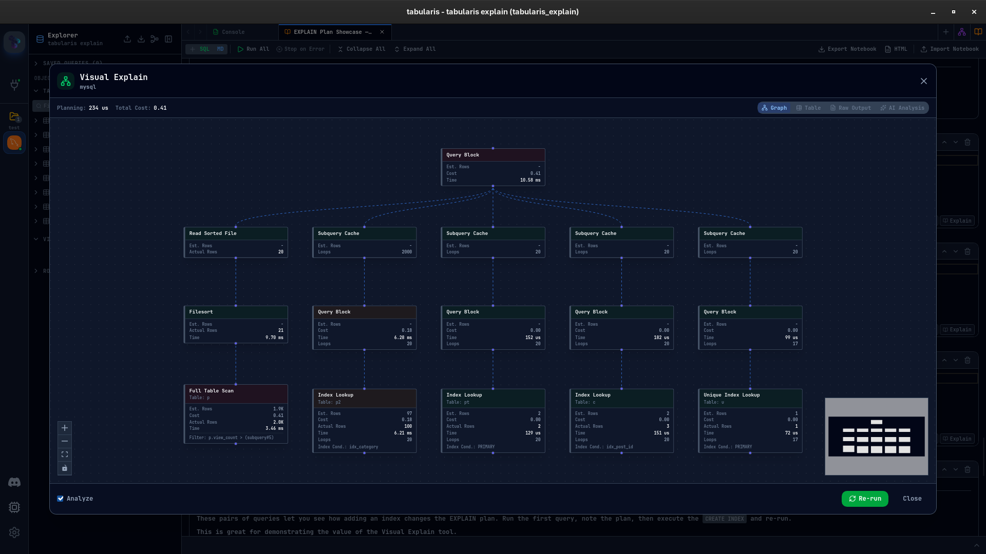
Table View
Better when you need exact numbers. The left panel is an expandable tree table with columns for node type, relation, cost, estimated rows, time, estimate gap, and filter. All nodes start expanded.
Selecting a row opens the detail panel on the right, which displays every metric available for that node: cost breakdown (startup to total), actual vs estimated rows, loops, buffer hits and reads, index conditions, hash conditions, join types, and any engine-specific fields.
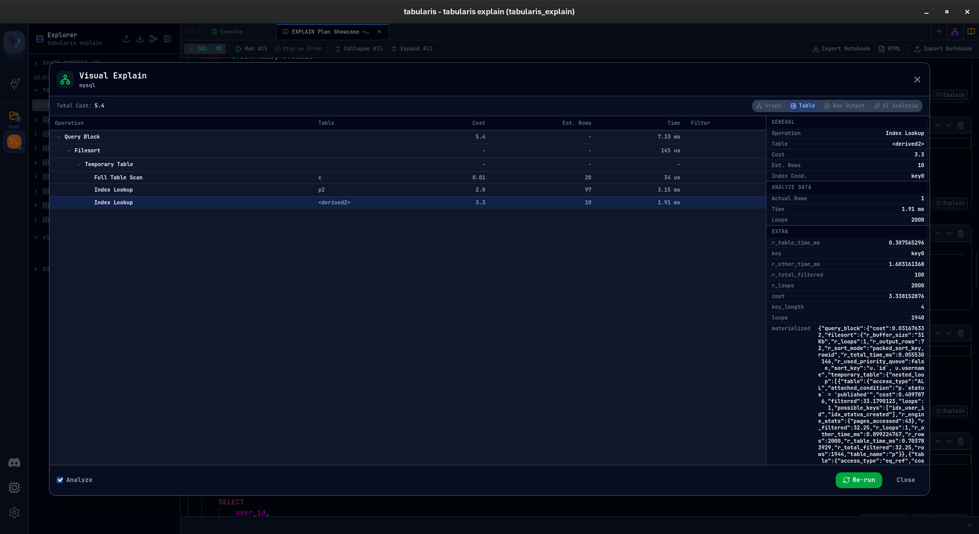
When the plan comes from EXPLAIN ANALYZE (or MariaDB ANALYZE), an Actual Rows column appears next to Est. Rows, so you can see where the optimizer's estimate diverged from what the query actually scanned.
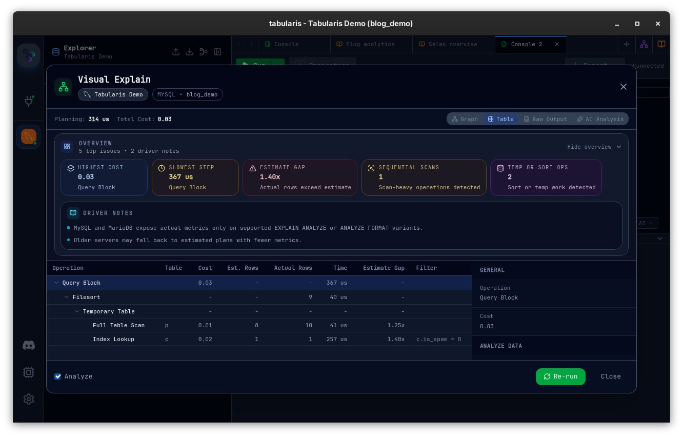
Diagram View
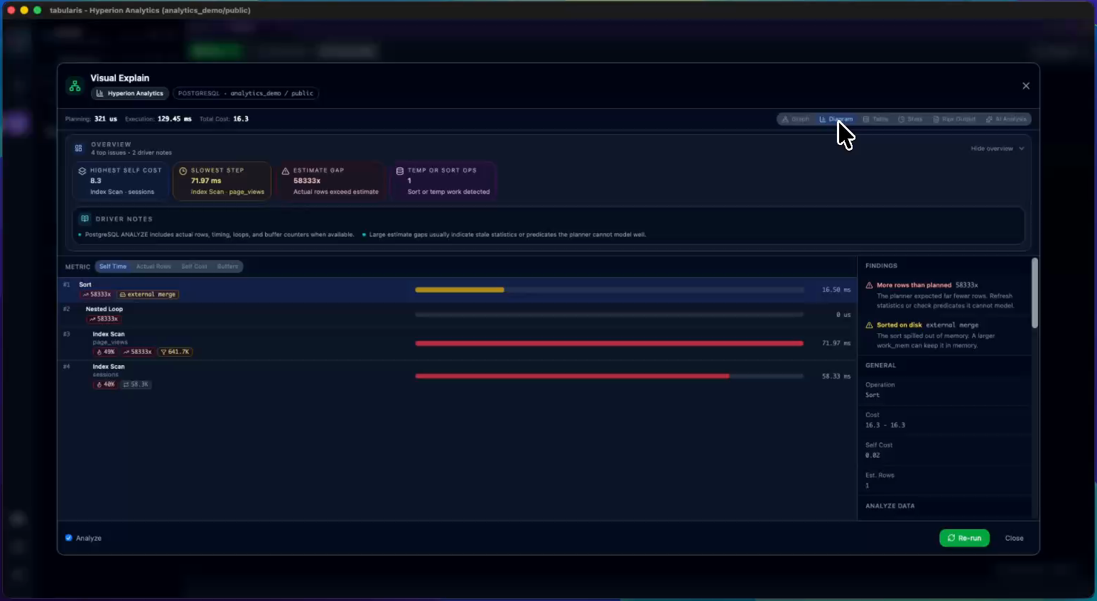
One row per node in plan order: index number, indentation showing the tree structure, node type and relation, a bar proportional to the selected metric, and the formatted value. The metric switches between time, rows, cost, and buffers — only metrics the plan actually carries are offered, defaulting to time when ANALYZE data is present and cost otherwise. Selection is shared with the graph, so a node picked in one view stays picked in the other.
Stats View
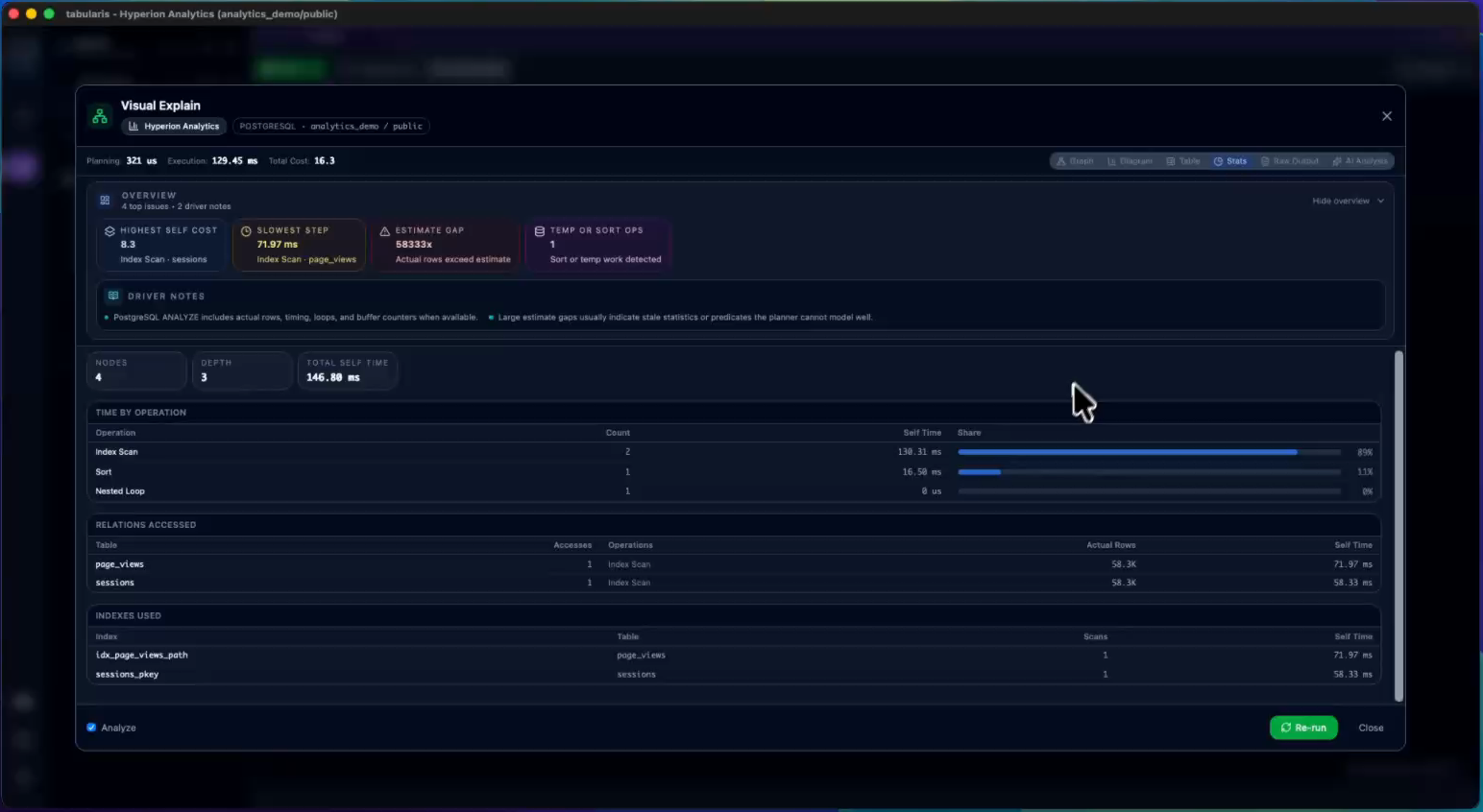
Plan-wide aggregates: node counts and depth, total self time, time by operation with share bars, relations accessed (access count, operations used, rows, self time), and indexes used with scan counts. Useful for answering "where does this plan spend its time" without walking the tree node by node.
Raw Output
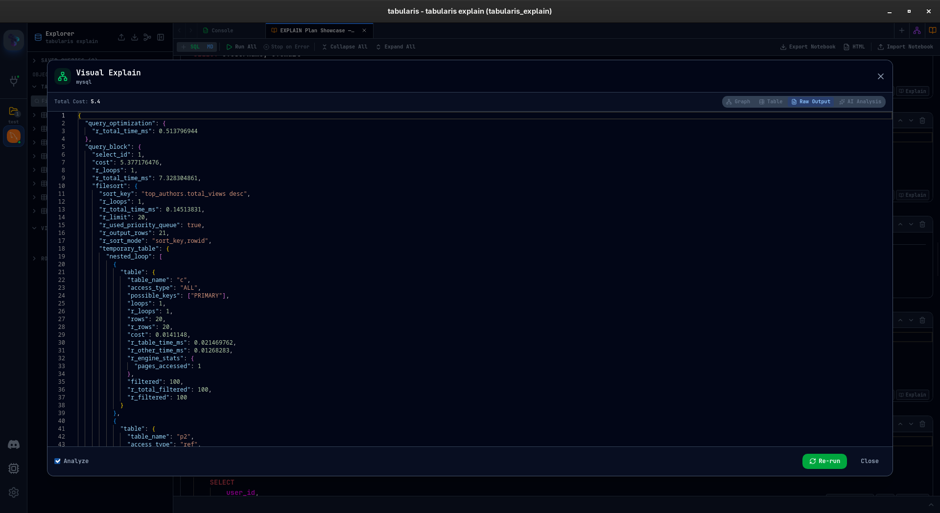
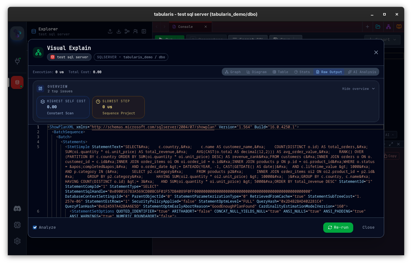
The raw view shows the database response in a read-only Monaco editor with syntax highlighting, word wrap, and search. No transformation — exactly what the server returned. JSON output from PostgreSQL or MySQL is detected automatically and highlighted as JSON; text-based output (like MySQL ANALYZE trees) renders as plain text. Since v0.23.0 XML plans are detected from the leading tag and highlighted as XML, and a single-line XML document (SQL Server SHOWPLAN output arrives this way) is indented one node per line for reading; already formatted XML passes through unchanged.
AI Analysis
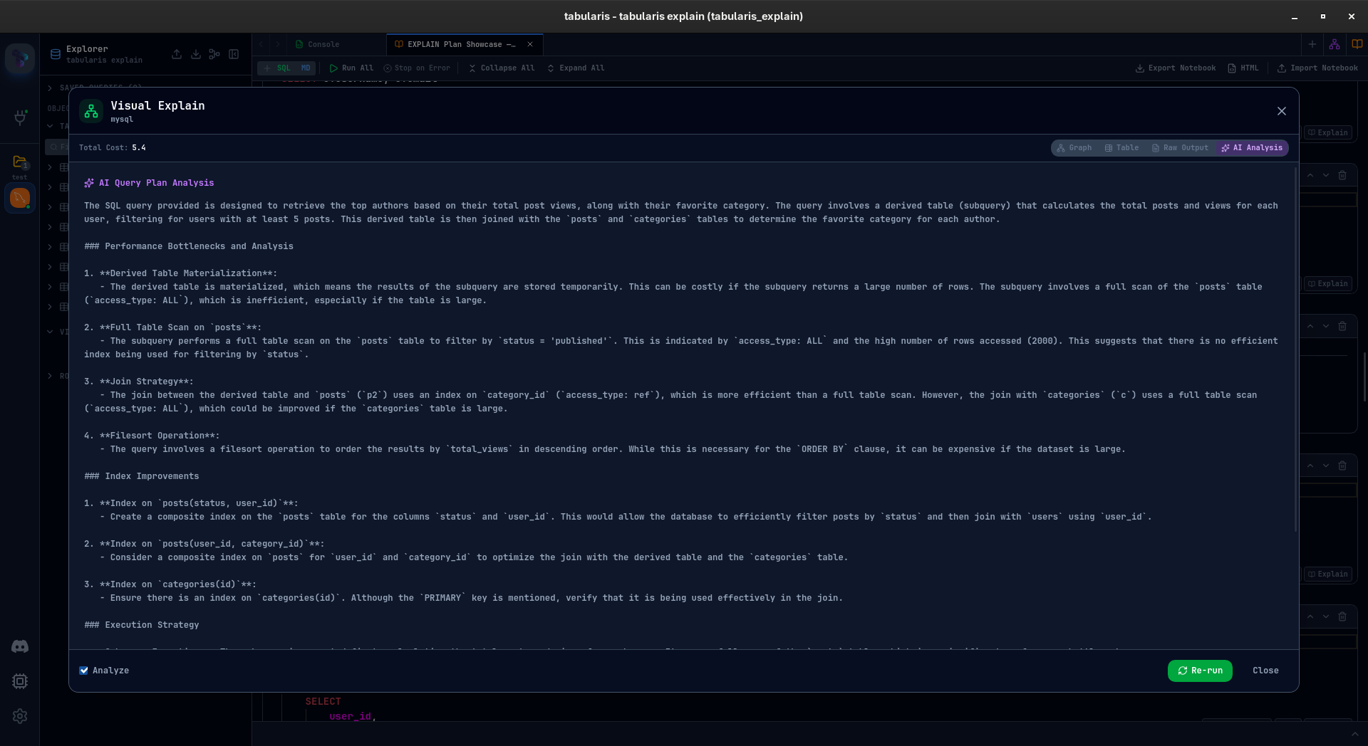
The AI tab sends the query and the raw EXPLAIN output to the configured AI provider and returns a structured analysis: what the query is doing, where the bottlenecks are, which indexes might help, and which rewrites are worth testing.
When you pick a language explicitly in Tabularis (any of the eleven supported UI languages, from Italian to Japanese to Korean), the analysis is generated in that language, so you do not need to reason about plans in English if that is not your working language. With the language set to Auto (the default), the analysis is always in English.
This tab only appears when AI is enabled in Settings > AI. If no AI provider is selected, the tab shows a warning above the analysis, which then fails. It works with all supported providers: OpenAI, Anthropic, Ollama, OpenRouter, MiniMax, and custom OpenAI-compatible endpoints.
The system prompt used for plan analysis can be customized in Settings > AI > Explain Plan Analysis Prompt.
Overview Bar
Below the summary bar, a collapsible Overview panel highlights the most relevant findings from the plan:
| Finding | What it shows |
|---|---|
| Highest Cost | The node with the largest exclusive (self) cost in the plan |
| Slowest Step | The node with the highest exclusive (self) execution time (only with ANALYZE) |
| Largest Estimate Gap | The node where the optimizer's row estimate was furthest from reality |
| Sequential Scans | Count of full table scans in the plan |
| Temp Operations | Count of sort, filesort, or temporary table operations |
Each finding is a clickable card — click it to select the corresponding node in the graph or table view and jump to its details. Below the findings, Driver Notes explain engine-specific context (e.g., what data is available with PostgreSQL ANALYZE vs MySQL EXPLAIN FORMAT=JSON).
Node Detail Panel
The detail panel appears on the right side of the graph, diagram and table views. It shows these sections for the selected node:
- Findings — the per-node findings described above, each with a one-line explanation
- General — node type, relation, cost (startup to total), estimated rows, filter, index condition, join type, hash condition
- Analyze Data — actual rows, actual time, loops, buffers hit, buffers read (only when ANALYZE was used)
- Extra Details — any additional fields from the engine that don't fit the standard categories (e.g., MariaDB's
r_filtered, MySQL'susing_temporary_table)
Database Support
Visual EXPLAIN adapts to each database engine. The differences between engines are handled automatically — you don't need to configure anything.
PostgreSQL
The most complete implementation. Tabularis runs EXPLAIN (FORMAT JSON, ANALYZE, BUFFERS) and parses the structured JSON output. Available metrics include planning time, execution time, buffer hit/read statistics, and the full node tree with both estimated and actual values.
If you are connected to a specific schema, search_path is set before running EXPLAIN so the plan reflects the correct schema context.
MySQL
MySQL support depends on the server version. Tabularis runs SELECT VERSION() and picks the best available format:
| Version | What Tabularis uses | Actual data? |
|---|---|---|
| MySQL 8.0.18+ | EXPLAIN ANALYZE (text tree) |
Yes |
| MySQL 5.6+ | EXPLAIN FORMAT=JSON |
No (estimates only) |
| Older versions | Tabular EXPLAIN |
No |
Version detection is automatic.
MariaDB
MariaDB is detected from the version string and uses its own syntax:
| Version | What Tabularis uses | Actual data? |
|---|---|---|
| MariaDB 10.1+ | ANALYZE FORMAT=JSON |
Yes (with r_* fields) |
| MariaDB 10.1+ | EXPLAIN FORMAT=JSON (fallback) |
No |
MariaDB's JSON format includes additional fields like subquery cache status, filesort details, and query optimization time. These appear in the Extra Details section of the node detail panel.
SQLite
SQLite uses EXPLAIN QUERY PLAN, which returns a flat list of operations. Tabularis reconstructs the tree structure from the parent-child relationships in the output.
SQLite does not expose execution metrics — there is no ANALYZE equivalent for query plans. The plan structure is shown (scan types, index usage, join order), but timing and row count data are not available. The ANALYZE toggle is accepted but has no effect.
Plugin Drivers
Plugin drivers opt in to Visual EXPLAIN through the explain capability flag in their .tabularium manifest. When a plugin declares "explain": true and implements the explain_query method, the EXPLAIN button and the editor context-menu entry work exactly as they do for the built-in drivers.
For drivers that do not declare the capability — or omit it entirely — the Visual EXPLAIN button is hidden in the SQL editor and in notebook cells, so you will only see it on connections that can actually produce a plan. See Plugin System for the full capability reference and Plugin Protocol for the explain_query method.
Since v0.23.0 a plugin no longer has to pre-parse its plan into the host's node shape. explain_query may return a raw result (engine, format and payload strings), and the plugin declares a matching TypeScript parser bundle in the explain_parsers array of its .tabularium manifest. Tabularis loads the bundle at runtime and registers it in the @tabularis/explain parser registry alongside the built-in PostgreSQL, MySQL and SQLite parsers, so the Graph, Table, Diagram, Stats, Raw and AI views work unchanged. Disabling and re-enabling the plugin unregisters and reloads its formats. Plugins that keep returning the parsed plan shape are unaffected. A plugin using the raw shape must declare min_runtime_version 0.23.0 or later; older hosts refuse it at install and load time instead of failing inside Visual EXPLAIN. The SQL Server plugin is the first to use this, with a sqlserver-showplan-xml parser; the design is described in How plugins can now inject their own parsers into Visual EXPLAIN and the manifest contract in EXPLAIN Parser Bundles.
Re-running a Plan
Click the Re-run button in the footer to execute the EXPLAIN again with the current settings (same query, same ANALYZE toggle state). This is useful after you've made changes — created an index, rewritten a join, or adjusted server configuration — and want to compare the new plan.
Notes
- The modal remembers your view mode selection while it's open. Switching between Graph, Table, Diagram, Stats, Raw, and AI does not re-run the query.
- Plans from
EXPLAIN ANALYZEon PostgreSQL include buffer statistics (shared hits and reads), which help distinguish between cached and disk I/O operations. - For large plans with many nodes, the graph view may need zooming. Use the fit-to-view control in the bottom-left corner to see the full tree.
- The AI analysis is a second-pass interpretation of the plan. It is not a replacement for understanding the execution plan yourself, but it can point you toward issues that are not immediately obvious in a large or unfamiliar plan.